Validating participant color response data

library(synr)

Why validate?

Clearly invalid data

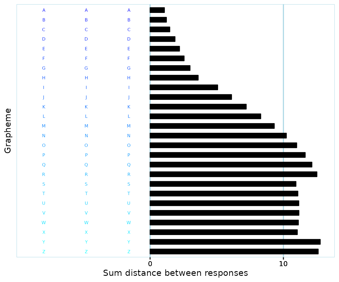
When conducting consistency tests with participants, there might be issues with their response patterns. A clear example of this is if a participant responds with a red color in all but two trials of a consistency test, like this:

This would lead to a very low (i. e. very consistent) consistency score. Should this score, and the data, be considered valid? Most synesthesia researchers would say no, and everyone would definitely say no if the participant themselves don’t report that they associate the color red with the stimuli used in the test.

Another instance of invalid data would be a participant who has provided ‘no color’ (if a ‘no color’/‘null’/‘blank’ response alternative is provided in the test) color responses for all but three graphemes. Even if the participant would have used one color for each grapheme and thus be very consistent, there’s a high risk that the participant simply memorized their previous responses throughout the test since they would have only had three graphemes to keep track of.

Clearly valid data

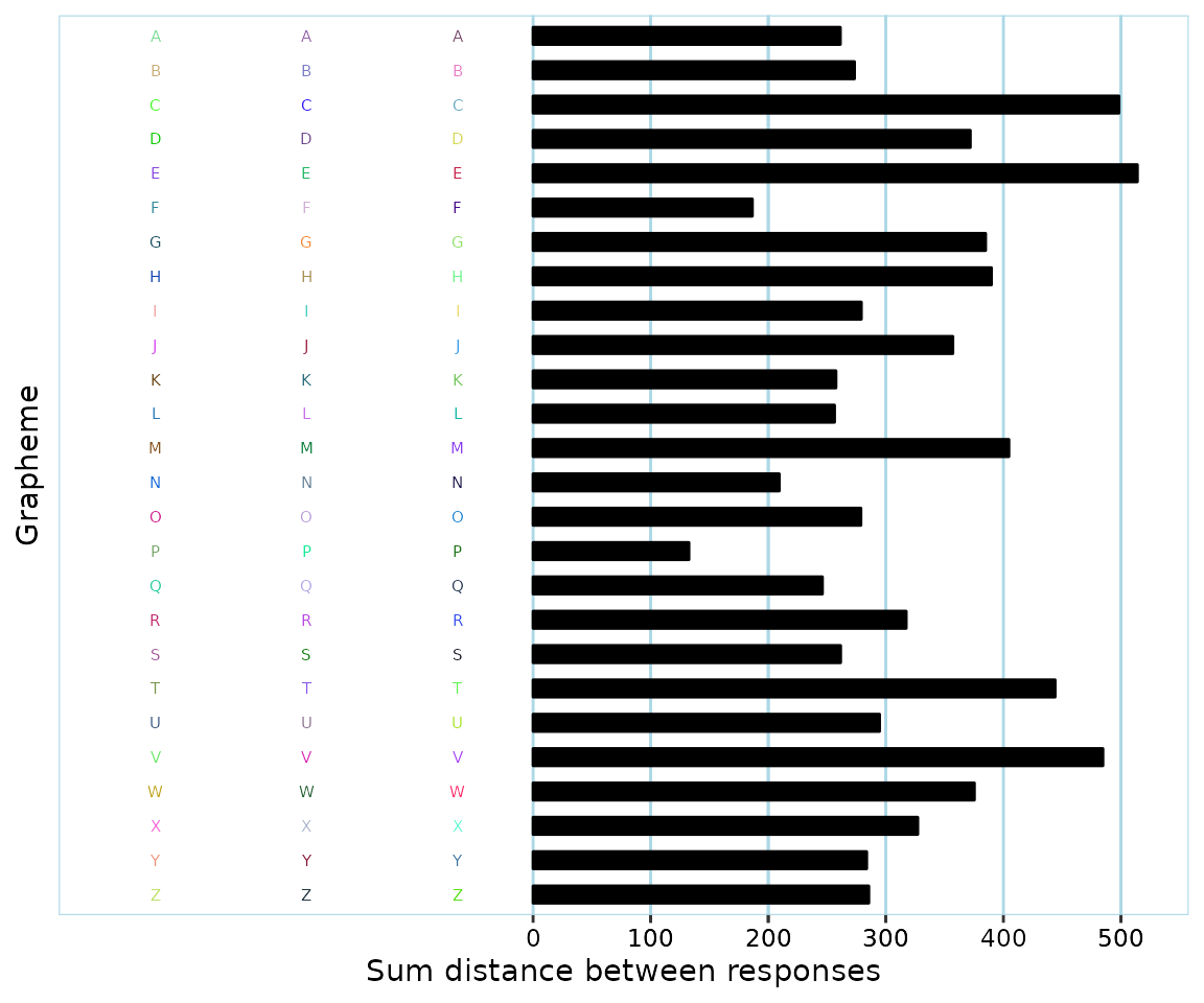
A clear example of valid response data is if a participant has used very different colors, like this:

Possibly invalid data

Many participants have response patterns that are harder to judge as valid or invalid, such as participants who have:

Used a red color for just 50% of all trials.
Used different shades of red and yellow for 90% of all trials.
Used black, white and blue for all trials.

Should some or all of these be considered to be examples of invalid data? Opinions are bound to differ.

Why validate: summary

The basic issue is that participants might give responses that vary too little in color for the consistency scores to mean anything. It is of course at least theoretically possible that someone would truly only have synesthetic associations with a single color. The consistency test, however, cannot determine whether this is the case, or if the participant for instance just likes the color red and keeps responding with it since that’s the color that comes to mind if they don’t have a stimulus-specific association.

Previously used validation procedures

Different research studies have handled possibly invalid data differently. Some (e.g. Cuskley et al., 2019) have opted for excluding participants which respond with ‘no color’ for more than a certain proportion of all trials. Others (Carmichael et al., 2015; Simner et al., 2006) have opted for (also) excluding participants who respond with ‘the same color’ in too high a proportion of trials. Yet others have excluded participants based on patterns that are more difficult to systematically define, such as a pattern involving selecting “e.g. red for ‘R’, green for ‘G’ and blue for ‘B’” (Carmichael et al., 2015).

Data validation challenges

Excluding participants based on the proportion or number of missing and/or ‘no color’ responses is relatively straight-forward, though there is currently no widely agreed upon threshold.

Excluding participants based on responses that do have an actual color, but where there is too little ‘color variation’, raises difficult questions which are briefly discussed below.

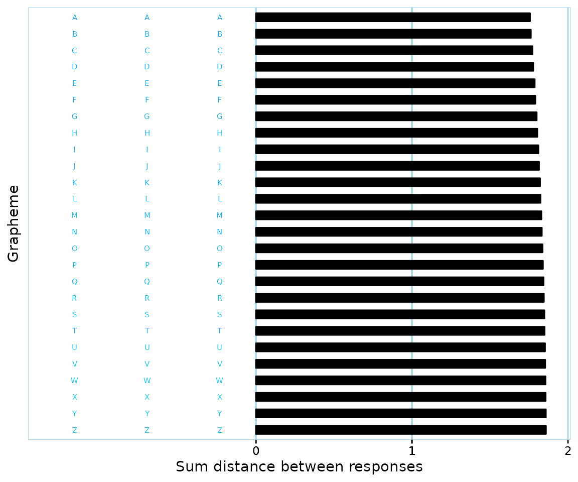
If using a criterion of allowing say only 60% of all responses to be of the ‘same color’, how does one define boundaries of what a color is? For instance, do teal, turquoise and cyan count as different colors? In the image below, where would you say that the ‘blue’ graphemes end, and the ‘blue-green’ graphemes start?

Even if one is able to consistently define color boundaries, what if a participant happens to respond with colors that are right at the ‘border’ of two color ranges? Relating back to the previous example, if you’ve defined where ‘blue’ ends and ‘bluegreen’ starts, a participant might give responses like this:

It might be reasonable to have placed the color border between ‘blue’ and ‘blue-green’ somewhere right around the middle of the above values. If categorizing response colors based on these boundaries, then, the participant would be considered to have 50% ‘blue’, and 50% ‘blue-green’ responses. But the color differences are so small, that a human observer who doesn’t know anything about the color borders would probably say that the participant has only responded with one color.

Finding a general validation procedure

Simple measures of spread

In order to get away from the arbitrariness of pre-defined ‘color ranges’, as discussed above, one option would be to use a general measurement of ‘spread’, similar to how we generally use variance and standard deviation in statistics. One might consider response colors as points in 3D color space, with e.g. axes ‘red’, ‘blue’ and ‘green’ (if using RGB color space). An example of this can be seen in the interactive graph below. Once you think of color data in this manner, it makes sense to base measures of spread on the distances between color points. A very simple approach might be to:

Calculate where the ‘middle’ (‘center of gravity’) of all points is located. (in the interactive graph below, the ‘middle’ is marked with a black point)
For each measured color point, calculate its distance from the ‘middle’.
Add up all these distances and divide by the total number of color points.

This would give a measure of spread based on the ‘mean distance from center of gravity (midpoint)’. To achieve something more analogous to variance as used with one-dimensional data, one may use squared distances from the ‘middle’ in steps 2 and 3. If you’re interested in the details of these calculations, see ‘More information’ at the end of this article.

The problem with simple measures of spread is that they are very sensitive to outliers and don’t take into account that responses might be ‘grouped together’. For instance, consider a participant who has given black color responses 80% of the time, and white color responses the rest of the time. To a human observer, it would appear that the participant has used a black color far too much for the data to say anything. But simple measures of spread would indicate that the participant response colors are very varied; since black and white are extreme opposites, the ‘middle’ will end up quite far from both groups of responses, and hence the (squared) distances will be long.

Clustering

One way to take into account that there might be patterns to response colors is to use so-called clustering (Jain, 2010). This is a general statistical approach for identifying groups of data that belong together and includes a number of specific methods, such as ‘k-means clustering’ and ‘Density-based spatial clustering of applications with noise’ (DBSCAN; Khan et al., 2014). DBSCAN is a good fit for grouping color responses since it doesn’t make any assumptions about the shape or number of clusters. See ‘More information’ at the end of this article to find out more about DBSCAN itself.

To understand what clustering and specifically DBSCAN does with color data, visualization helps. Let’s say a participant has a set of response colors as described by this interactive graph:

To a typical human observer, it looks like there are groups of black, red and white color responses, respectively. Apart from these, there are a few color responses that don’t seem to be part of a particular pattern. (the white color points are hard to make out in the graph because of the white background - it might help to touch/hover with your mouse around the ‘white corner’ to have them highlighted)

Applying DBSCAN and recoloring color points according to what cluster they belong to, the result might look something like this:

The following clusters have been identified:

Cluster 0: ‘noise’ cluster, which includes all points that weren’t included in a specific cluster.
Cluster 1: white color responses (presented in dark blue).
Cluster 2: intensely red color responses (presented in a blue-green color).
Cluster 3: black color responses (presented in green).
Cluster 4: red, but less intense, color responses (presented in a yellow color).

You might need to go back and forth a few times between the previous two graphs for them to make sense.

We might agree with how DBSCAN clustered together ‘white’ (cluster 1) and ‘black’ (cluster 3) color points, respectively. Depending on how you perceive and define colors, you might agree or disagree with how the ‘red’ color points were grouped into two separate clusters. The point is that using DBSCAN, one can be explicit about how color points should be clustered together instead of relying on post-hoc subjective judgments or arbitrary pre-defined ‘color borders’ as discussed earlier. How this clustering happens is primarily determined by ‘epsilon’ (eps) and ‘minimum points in cluster’ (minPts) parameters - see the ‘More information’ section.

DBSCAN on its own is however not sufficient for validating color response data. The reason is that it doesn’t take into account what happens ‘within’ clusters. A participant might vary their responses so much that they all end up in the ‘noise’ cluster. Or, they might have responses similar to what’s seen below:

DBSCAN would consider all of the above points to form a single cluster, since every single point has at least one ‘neighbor’ linking it to the greater cluster. Granted, it’s unlikely that a participant will respond in this particular manner, but the same phenomenon of fairly spread out points being ‘chained together’ does happen in real data. Thus, simply counting the number of clusters isn’t enough to be able to determine the validity of color response data.

Combining measure of spread and DBSCAN

In order to take into account all relevant information, synr uses an approach for validating participant data that is based on combining DBSCAN and the ‘variance-like’ measure of spread described earlier.

As part of the validation procedure, synr calculates total within-cluster variance (TWCV). This is a modified measure of the data’s total variance that takes into account clustering of data. You can find details about this by reading the help documentation for the synr total_within_cluster_variance function.

What follows is a rough overview of an example of synr’s validation procedure being applied. It is assumed that participant data are from a consistency test where each grapheme was presented for 3 trials. Many aspects of the validation are specified by you as the user, but example values (marked in bold) are used to make the example more concrete.

If a participant has less than 6 graphemes with complete color responses (3 color responses that aren’t of type ‘blank’/‘no color’), their data are directly classified as invalid.
Data from graphemes with non-complete color responses are filtered away.
DBSCAN is applied to find clusters of color points in the ‘complete grapheme’ data.
The ‘variance’ of each cluster is calculated.
The TWCV is calculated.
If a single low-variance cluster, ie a ‘tight-knit’ cluster, includes more than 60% of all color points, the participant data are classified as invalid.

Once steps 1-6 are cleared:

If DBSCAN identified 4 or more clusters (roughly meaning that 4 or more colors were each used for multiple responses), the participant data are classified as valid.
If the TWCV score was 250 or more, the participant data are classified as valid.

In other words, if the participant data had few clusters, and their TWCV score was below 250, they are classified as invalid.

This approach enables invalidating data from participants who used one or just a few colors too much, while still validating different valid patterns of responding.

Applying synr’s validation procedure, `check_valid_get_twcv_scores`

You first need a participantgroup (see the quickstart/main tutorial if this is new to you)

# if you don't already have synr loaded, run 'library(synr)' first
pg <- create_participantgroup(
  raw_df=synr_exampledf_large,
  n_trials_per_grapheme=3,
  id_col_name="participant_id",
  symbol_col_name="trial_symbol",
  color_col_name="response_color",
  time_col_name="response_time", # optional, not necessary for core functionality
  color_space_spec="Luv"
)

Note that the color space specification (color_space_spec) will also affect synr’s validation procedure. It is recommended that you use CIELUV (‘Luv’) or some other color space that aims to be in line with human perception. You might have noticed that RGB was used in the interactive graphs earlier as it’s fairly intuitive, but it is not suitable for validation procedures.

Now that you have a participantgroup, you want to use the check_valid_get_twcv_scores method. This applies a validation procedure, similar to the one outlined above, on a per-participant basis for all participants in the group. The method’s parameters and output are explained below.

set.seed(1)
val_df <- pg$check_valid_get_twcv_scores(
  min_complete_graphemes = 4,
  dbscan_eps = 20,
  dbscan_min_pts = 4,
  max_var_tight_cluster = 150,
  max_prop_single_tight_cluster = 0.6,
  safe_num_clusters = 3,
  safe_twcv = 250,
  complete_graphemes_only = TRUE,
  symbol_filter = LETTERS
)

head(val_df)
#>   valid        reason_invalid      twcv num_clusters
#> 1  TRUE                       1077.9557            8
#> 2 FALSE hi_prop_tight_cluster  195.1215            2
#> 3  TRUE                       1222.0226            5
#> 4  TRUE                       1568.6686            5
#> 5  TRUE                       3154.0720            4

Parameters

min_complete_graphemes The minimum number of graphemes with complete (all non-NA color) responses that a participant’s data must have for them to not be categorized as invalid based on this criterion.
dbscan_eps Radius of ‘epsilon neighborhood’ when applying DBSCAN clustering.
dbscan_min_pts Minimum number of points required in the epsilon neighborhood for core points (including the core point itself) when applying DBSCAN clustering.
max_var_tight_cluster Maximum variance for an identified DBSCAN cluster to be considered ‘tight-knit’.
max_prop_single_tight_cluster Maximum proportion of color points allowed to be within a single ‘tight-knit’ cluster (if a participant’s data exceed this limit, they are classified as invalid).
safe_num_clusters Minimum number of identified DBSCAN clusters (including the ‘noise’ cluster if it consists of at least dbscan_min_pts points) that guarantees validity of a participant’s data if points are ‘non-tight-knit’.
safe_twcv Minimum total within-cluster variance (TWCV) score that guarantees a participant’s data’s validity if points are ‘non-tight-knit’.
complete_graphemes_only If TRUE, only data from graphemes with complete sets of associated color responses are used for clustering and variance calulations. If FALSE, even data from graphemes with ‘incomplete’ response data are included.
symbol_filter A character vector (or NULL) that specifies which graphemes’ data to use. If NULL, data from all of the participants’ graphemes (apart from filtering based on complete response data) will be used.

Output A data frame with columns:

valid Holds TRUE for participants whose data were classified as valid, FALSE for participants whose data were classified as invalid.
reason_invalid Strings which describe for each participant why their data were deemed invalid. Participants whose data were classified as valid have empty strings here.
twcv Numeric column which holds participants’ calculated TWCV scores.
num_clusters Numeric column which for each participant holds the number of identified clusters (including the ‘noise’ cluster if it consists of at least dbscan_min_pts points).

Note the set.seed(1) call. This is necessary for replication. DBSCAN uses a partially random procedure for determining clusters. In practice, when this has been tested by the main developer (see below), the results have always been the same, but for some very unusual sets of data the results might differ. Hence, set.seed(<number>) should always be included in any code you save/share, to be absolutely certain that check_valid_get_twcv_scores will produce the same output if run again.

Similar to other synr methods’ outputs, in order to tell which classification goes with which participant, combine the output with results from get_ids.

val_id_df <- cbind(list(participant_id=pg$get_ids()), val_df)

head(val_id_df)
#>   participant_id valid        reason_invalid      twcv num_clusters
#> 1          partA  TRUE                       1077.9557            8
#> 2          partB FALSE hi_prop_tight_cluster  195.1215            2
#> 3          partC  TRUE                       1222.0226            5
#> 4          partD  TRUE                       1568.6686            5
#> 5          partE  TRUE                       3154.0720            4

Parameter values and previous applications of synr’s data validation

The approach of using DBSCAN together with 3D ‘variance’ scores for validation of consistency test data is, so far, unique to synr. Thus, there are no norms regarding what particular values should be used.

The main developer of synr (Lowe Wilsson) has applied check_valid_get_twcv_scores to a sample of consistency test data from 268 participants with the exact values specified in the example above, and then compared the results to independent classifications by human raters. The data in the sample included digit and letter graphemes, where each grapheme had been used in 3 trials. Classifications were made separately for the digit and letter categories.

The validity criteria used by human raters in the example sudy were chiefly that participants needed to have at least 4 graphemes with ‘complete responses’ (ie 3 non-‘blank’ color responses) in the category being considered, that they used at least three different colors (eg yellow, red, orange), and that they didn’t use the same color for more than 60% of all responses.

When classifications produced by synr were compared with those of human raters, there was agreement for all but a handful of participants. In most of these cases, it turned out that the human raters had missed some detail, eg participants who had used the same color for just over 60% of all responses had been erroneously classified as valid. In one case, a participant had responded with different shades of red that were somewhat close to orange, leading to a disagreement among the human raters. In the end, after discussion the consensus was that synr’s classifications were the most accurate in all cases.

Summary

synr uses a novel approach for validating participant data which shows great promise. It is likely to reduce time spent on manually sorting through consistency test data. Most of all, it lets researchers clearly specify and operationalize valid data criteria. The procedure involves more abstract concepts like ‘total within-cluster variance’, but has the benefit of not having to rely on diffuse concepts like ‘number of colors’.

Note that a synr ‘invalid’ classification essentially means that it’s inappropriate to simply feed the data into consistency scoring algorithms. It’s up to users to decide how to handle participants with ‘invalid’ data, eg by excluding them from analyses entirely or considering them as non-synesthetes.

Some response patterns only make sense to humans and cannot be picked up by DBSCAN. An example is using an __o__range color for the grapheme ‘O’, which was found in one study (Simner et al., 2006) to be more frequent among self-reported non-synesthetes with low consistency scores than among self-reported synesthetes. If validity assessments are to take these very subjective patterns into account (as done in e. g. Carmichael et al., 2015), synr needs to be complemented by human ratings.

If synr is used for data validation then please reference synr itself (for now, https://cran.r-project.org/package=synr) and include code and/or values you passed to check_valid_get_twcv_scores when reporting results. It’s also important to avoid post-hoc definitions of validation criteria. Thus, if it’s feasible, please decide before starting data collection, or based on a smaller initial sample, what values to use with check_valid_get_twcv_scores.

More information

DBSCAN

3-minute YouTube video giving a brief introduction to DBSCAN: https://www.youtube.com/watch?v=_A9Tq6mGtLI.

Official documentation for the dbscan package: https://www.rdocumentation.org/packages/dbscan/versions/1.1-8

Apart from the above sources, if you are new to clustering you might find it helpful to search for introductory material on clustering in general, and multiple visualizations of applying DBSCAN specifically. In particular, the documentation for the dbscan package might not make much sense until you understand the theoretical background.

Data validation in synr

More details about data validation-related procedures can be found in synr’s documentation for the following functions (access the documentation by running e.g. ?synr::centroid_3d_sq_dist):

centroid_3d_sq_dist
total_within_cluster_variance
validate_get_twcv

You can also find higher-level information in the documentation for the check_valid_get_twcv_scores method by running ?synr::ParticipantGroup.

References

Carmichael, D. A., Down, M. P., Shillcock, R. C., Eagleman, D. M., & Simner, J. (2015). Validating a standardised test battery for synesthesia: Does the Synesthesia Battery reliably detect synesthesia? Consciousness and Cognition, 33, 375–385.

Cuskley, C.1, Dingemanse, M.1, van Leeuwen, T. & Kirby, S. 2019. Cross-modal associations and synaesthesia: Categorical perception and structure in vowel-colour mappings in a large online sample. Behaviour Research Methods, doi: 10.3758/s13428-019-01203-7

Khan, K., Rehman, S. U., Aziz, K., Fong, S., & Sarasvady, S. (2014). DBSCAN: Past, present and future. The Fifth International Conference on the Applications of Digital Information and Web Technologies (ICADIWT 2014), 232–238.

Jain, A. K. (2010). Data clustering: 50 years beyond K-means. Pattern Recognition Letters, 31(8), 651–666.

Simner, J., Mulvenna, C., Sagiv, N., Tsakanikos, E., Witherby, S. A., Fraser, C., Scott, K., & Ward, J. (2006). Synaesthesia: The prevalence of atypical cross-modal experiences. Perception, 35(8), 1024–1033.